Friday, December 23, 2011

Scrabbling with Shannon

Once the AI Class was over, I wanted to take some time to study the second optional NLP problem with Python. Finding a solution is not difficult (because even an imperfect one will yield the answer anyway), but devising a satisfying process to do so (i.e. a general way of solving similar problems), is much harder.

Problem Representation

The first task is working up the problem representation. We need to parse:

s = """|de|  | f|Cl|nf|ed|au| i|ti|  |ma|ha|or|nn|ou| S|on|nd|on|
       |ry|  |is|th|is| b|eo|as|  |  |f |wh| o|ic| t|, |  |he|h |
       |ab|  |la|pr|od|ge|ob| m|an|  |s |is|el|ti|ng|il|d |ua|c |
       |he|  |ea|of|ho| m| t|et|ha|  | t|od|ds|e |ki| c|t |ng|br|
       |wo|m,|to|yo|hi|ve|u | t|ob|  |pr|d |s |us| s|ul|le|ol|e |
       | t|ca| t|wi| M|d |th|"A|ma|l |he| p|at|ap|it|he|ti|le|er|
       |ry|d |un|Th|" |io|eo|n,|is|  |bl|f |pu|Co|ic| o|he|at|mm|
       |hi|  |  |in|  |  | t|  |  |  |  |ye|  |ar|  |s |  |  |. |"""

A useful data structure in this context is a list of 19 sublists, each corresponding to a column of 8 tokens. The reason for this is that we need to easily shuffle around the columns, which are the atomic parts of the problem (i.e. those which cannot change):

grid = [[''] * 8 for i in range(19)]
for j, line in enumerate(s.split('\n')):
    cols = line.strip().split('|')[1:-1]
    for i, col in enumerate(cols):
        grid[i][j] = col

There are certainly more elegant ways to handle this, but this is enough for the discussion. To revert back from this representation to a readable form:

def repr(grid):
    return '\n'.join(['|%s|' % '|'.join([grid[i][j] for i in range(19)]) for j in range(8)])

We need to consider two abstract components for solving this problem: the state space exploration, and the evaluation function we must use to guide it, since there's clearly no way we can brute-force the 19! possible configurations.

State Space Exploration

For the exploration function, here is a simple approach: from a given grid configuration, consider all the possible grid reorderings, resulting from having an arbitrary column reinserted to an arbitrary position. Then expand them in the order of their score ranking. Here is an example showing two possible column reorderings from the initial state:
Note that this is not the same as simply swapping columns: from "a,b,c", for instance, we'd like to derive "b,a,c", "b,c,a", "c,a,b" and "a,c,b", which wouldn't possible with only one swapping step. One way to do this is:

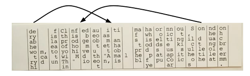
def nextGrids(grid):
    global visited # I know..
    next_grids = set()
    for i in range(19):
        for j in range(19):
            if i == j: continue
            next_grid = list(list(col) for col in grid)
            next_grid.insert(i, next_grid.pop(j))
            next_grid = tuple(tuple(col) for col in next_grid)
            if next_grid not in visited:
                next_grids.add(next_grid)
    return next_grids

Again it's quite certain that nicer solutions exist for this: in particular, I use sets to avoid repetitions (both for the already explored states overall and the reinsertion configs for a given grid), which thus requires those ugly "tuplify/listify" operations (a list is editable but not hashable, while a set is the opposite). We can then use this function in a greedy and heuristic way, always expanding first the best reordering from any given state (using a heap to make our life easier):

visited = set()
frontier = [] # heap of (score, grid)'s
while True:
    for next_grid in nextGrids(grid):
        # using a min-heap so score has to be negated
        heappush(frontier, (-gridScore(next_grid), next_grid))
    score, grid = heappop(frontier)
    visited.add(grid)
    score, grid = max(results)
    print repr(grid)
    print score

This is obviously greedy, because it might easily overlook a better, but more convoluted solution, while blindly optimizing the current step. Our only hope is that the evaluation function might be more clever in compensation. Note also that we don't stop, simply because there is no obvious criterion for doing so. We could define a tentative one, but since that's not the goal of the exercise, let's just proceed by inspection (once I knew the answer, I cheated by hardcoding a stopping criterion, just for the purpose of counting the number of steps to reach it). But then what about the scores? But just before..

Some Doubts..

At first, my solution wasn't based on a heap: it was simply considering the best configuration at any point, and then would forget about the others (in other words: it used a single-element search frontier). But I had doubts: was this strategy guaranteed to eventually exhaust the space of the possible permutations of a given set? If not, even in theory, it would seem to be a potential problem as for the generalness of the solution.. I'm not sure about the math required to describe the relationship between the n! permutations of a set and the n2-2n+1 element reorderings (there must be a technical term for this?) from any configuration, but after having performed some practical tests, I reached the conclusion that using a heap-based method (i.e. a frontier with many elements) was more sound, because although I cannot prove it, I'm pretty certain that it is guaranteed to eventually exhaust the permutation space, whereas the first method is not. In the context of this problem, it doesn't make a difference though, because the search space is so large that we would have to wait a very long time before we see these two closely related strategies behave differently.

Language Modeling

Enters language modeling.. this is the component we need for the evalution function, to tell us if we are heading in the right direction or not, in terms of unscrambling the hidden message. My first intuition was that character-based n-grams would work best. Why? Because while exploring the state space, due to the problem definition, most of the time we are dealing with parts or scrambled words, not complete (i.e. real) ones. Thus a character-based n-gram should be able to help, because it works at the sub-lexical level (but happily not exclusively at this level, as it retains its power once words begin to get fully formed, which is what we want). To do this, I used the venerable Brown Corpus, a fairly small (by today's standards) body of text containing about 1M words, which should be enough for this problem (note that I could have also used NLTK):

CHAR_NGRAM_ORDER = 3
EPSILON = 1e-10
char_counts = defaultdict(int)
for line in open('brown.txt'):
    words = re.sub(r'\W+', ' ', line).split() # tokenize with punctuation and whitespaces
    chars = ' '.join(words)    
    char_counts[''] += len(chars) # this little hack is useful for 1-grams
    for n in range(CHAR_NGRAM_ORDER):
        for i in range(len(chars)):
            if i >= n:
                char_counts[chars[i-n:i+1]] += 1

# charProb('the') should be > than charProb('tha')
def charProb(c):
    global char_counts
    if c in char_counts:
        return char_counts[c] / char_counts[c[:-1]]
    return EPSILON

Another debatable aspect: I use a very small value as the probability of combinations that have never been seen, instead of using a proper discounting method (e.g. Laplace) to smooth the MLE counts: I thought it wouldn't make a big difference, but I might be wrong. The outcome however is that I cannot talk about probabilities, strictly speaking, so let's continue with scores instead (which means something very close in this context).

The final required piece is the already mentioned function to compute the score for a given grid:

def gridScore(grid):
    # add spaces between rows
    s = ' '.join([''.join([grid[i][j] for i in range(19)]) for j in range(8)])
    # tokenize with punctuation and whitespaces
    s = ' '.join(re.sub(r'\W+', ' ', s).split()) 
    LL = 0 # log-likelihood
    for i in range(len(s)):
        probs = []
        for n in range(CHAR_NGRAM_ORDER):
            if i >= n:
                probs.append(charProb(s[i-n:i+1]))
        # interpolated LMs with uniform weights
        pi = sum([p/len(probs) for p in probs])
        LL += math.log(pi)
    return LL

A couple of things to note: I use the log-likelihood because it is more numerically stable, and I also use a simple interpolation method (with uniform weights) to combine models of different orders.

So.. does this work? Not terribly well unfortunately.. Although with some tuning (the most important aspect being the order N of the model) it's possible to reach somewhat interesting states like this:

    | i|nf|or|ma|ti|on|ed|Cl|au|de| S|ha|nn|on| f|ou|nd|  |  |
    |as|is| o|f |  |  | b|th|eo|ry|, |wh|ic|h |is| t|he|  |  |
    | m|od|el|s |an|d |ge|pr|ob|ab|il|is|ti|c |la|ng|ua|  |  |
    |et|ho|ds| t|ha|t | m|of| t|he| c|od|e |br|ea|ki|ng|  |  |
    | t|hi|s |pr|ob|le|ve|yo|u |wo|ul|d |us|e |to| s|ol|m,|  |
    |"A| M|at|he|ma|ti|d |wi|th| t|he| p|ap|er| t|it|le|ca|l |
    |n,|" |pu|bl|is|he|io|Th|eo|ry| o|f |Co|mm|un|ic|at|d |  |
    |  |  |  |  |  |  |  |in| t|hi|s |ye|ar|. |  |  |  |  |  |

from which it's rather easy to guess the answer (we are so good at this actually that there's even an internet meme celebrating it), for some reason my experiments seemed to always find themselves stuck in some local minima from which they could not escape.

The Solution

Considering the jittery nature of my simplistic optimization function (although you prefer it to go up, there is no guarantee that it will always do), I pondered for a while about a backtracking mechanism, to no avail. The real next step is rather obvious: characters are probably not enough, the model needs to be augmented at the level of words. The character-based model should be doing most of the work in the first steps of the exploration (when the words are not fully formed), and the word-based model should take over progressively, as we zero in on the solution. It's easy to modify the previous code to introduce this new level:

CHAR_NGRAM_ORDER = 6
WORD_NGRAM_ORDER = 1
char_counts = defaultdict(int)
word_counts = defaultdict(int)
for line in open('brown.txt'):
    # words
    words = re.sub(r'\W+', ' ', line).split() # tokenize with punctuation and whitespaces
    word_counts[''] += len(words) # this little hack is useful for 1-grams
    for n in range(WORD_NGRAM_ORDER):
        for i in range(len(words)):
            if i >= n:
                word_counts[' '.join(words[i-n:i+1])] += 1
    # chars
    chars = ' '.join(words)    
    char_counts[''] += len(chars)
    for n in range(CHAR_NGRAM_ORDER):
        for i in range(len(chars)):
            if i >= n:
                char_counts[chars[i-n:i+1]] += 1

# wordProb('table') should be > than wordProb('tabel')
def wordProb(w):
    global word_counts
    words = w.split()
    h = ' '.join(words[:-1])
    if w in word_counts:
        return word_counts[w] / word_counts[h]
    return EPSILON

def gridScore(grid):
    # add spaces between rows
    s = ' '.join([''.join([grid[i][j] for i in range(19)]) for j in range(8)])
    # tokenize with punctuation and whitespaces
    s = ' '.join(re.sub(r'\W+', ' ', s).split()) 
    LL = 0 # log-likelihood
    for i in range(len(s)):
        probs = []
        for n in range(CHAR_NGRAM_ORDER):
            if i >= n:
                probs.append(charProb(s[i-n:i+1]))
        if not probs: continue
        pi = sum([p/len(probs) for p in probs])
        LL += math.log(pi)
    words = s.split()
    for i in range(len(words)):
        probs = []
        for n in range(WORD_NGRAM_ORDER):
            if i >= n:
                probs.append(wordProb(' '.join(words[i-n:i+1])))
        if not probs: continue
        pi = sum([p/len(probs) for p in probs])
        LL += math.log(pi)
    return LL

After some tinkering, I found that character-based 6-grams augmented with word unigrams was the most efficient model, as it solves the problem in 15 steps only. Of course this is highly dependent on the ~890K training parameters obtained using the Brown corpus, as with some other text it would probably look quite different. I'm not sure if this is the optimal solution (it's rather hard to verify), but it should be pretty close.

And finally.. isn't it loopy in a strange way that the solution to a problem refers to what is probably the most efficient way of solving it?

That was really fun, as the rest of the course was, and if this could be of interest to anyone, the code is available on GitHub.

Tuesday, November 29, 2011

A Birthday Simulator

Earlier today I was reading about the Tuesday Birthday Problem (which curiously doesn't seem to have its own entry on Wikipedia.. maybe it is known under a different name?) and although I was convinced by the argument, I thought that a little simulation would help deepen my understanding of this strange paradox (or at least make it a little more intuitive). The problem I had is how to represent, in a clear way, some a priori knowledge (namely, the fact that one of the children is a son born on a Tuesday) in a numerical simulation?

Since directly modeling the conditional distribution wouldn't be trivial, an easier way to do it is by using rejection sampling: iterate over a set of randomly generated family configurations, and reject those that do not match the given fact, i.e. those not containing at least a son born on a Tuesday. From the configurations that passed the test, the proportion of those having the other child also a son (born on whatever day), should yield the answer (which of course is not 1/2, as intuition first strongly suggests):

from __future__ import division
from random import *

n = 0
n_times_other_child_is_son = 0
while n < 100000:
    child1 = choice('MF') + str(randint(0, 6))
    child2 = choice('MF') + str(randint(0, 6))
    children = child1 + child2
    if 'M2' not in children: continue
    if children[0::2] == 'MM':
        n_times_other_child_is_son += 1
    n += 1

print n_times_other_child_is_son / n # should be close to 13/27

Thursday, October 6, 2011

A Wormhole Through Sudoku Space

I did what I suggested in my last post, and finally read about Peter Norvig's constraint propagation method for solving Sudoku. On one hand it's quite humbling to discover a thinking process so much more elaborate than what I could achieve, but on the other, I'm glad that I didn't read it first, because I wouldn't have learned as much from it.

It turns out that my insights about search were not so far off the mark... but then the elimination procedure is the real deal (in some cases, it can entirely solve an easy problem on its own). In fact the real power is unleashed when the two are combined. The way I understand it, elimination is like a mini-search, where the consequences of a move are carried over their logical conclusion, revealing, many steps ahead, if it's good or not. It is more than a heuristic, it is a solution space simplifier, and a very efficient one at that.

My reaction when I understood how it worked was to ask myself if there's a way I could adapt it for my current Python implementation, without modifying it too much. It is not exactly trivial, because the two problem representation mechanisms are quite different: Peter Norvig's one explicitly models the choices for a given square, while mine only does it implicitly. This meant that I couldn't merely translate the elimination algorithm in terms of my implementation: I'd have to find some correspondence, a way to express one in terms of the other. After some tinkering, what I got is a drop-in replacement for my Sudoku.set method:

    def set(self, i, j, v, propagate_constraints):
        self.grid[i][j] = v
        self.rows[i].add(v)
        self.cols[j].add(v)
        self.boxes[self.box(i, j)].add(v)
        if propagate_constraints:
            for a in range(self.size):
                row_places = defaultdict(list) 
                row_available = set(self.values)
                col_places = defaultdict(list) 
                col_available = set(self.values)
                box_places = defaultdict(list) 
                box_available = set(self.values)
                for b in range(self.size):
                    options = []
                    row_available.discard(self.grid[a][b])
                    col_available.discard(self.grid[b][a])
                    bi, bj = self.box_coords[a][b]
                    box_available.discard(self.grid[bi][bj])
                    for vv in self.values:
                        if not self.grid[a][b] and self.isValid(a, b, vv):
                            options.append(vv)
                            row_places[vv].append(b)
                        if not self.grid[b][a] and self.isValid(b, a, vv):
                            col_places[vv].append(b)
                        if not self.grid[bi][bj] and self.isValid(bi, bj, vv):
                            box_places[vv].append((bi,bj))
                    if not self.grid[a][b]:
                        if len(options) == 0: 
                            return False
                        elif len(options) == 1:
                            # square with single choice found
                            return self.set(a, b, options[0], propagate_constraints)
                if row_available != set(row_places.keys()): return False
                if col_available != set(col_places.keys()): return False
                if box_available != set(box_places.keys()): return False
                for vv, cols in row_places.items():
                    if len(cols) == 1:                       
                        # row with with single place value found
                        return self.set(a, cols[0], vv, propagate_constraints)
                for vv, rows in col_places.items():
                    if len(rows) == 1:                        
                        # col with with single place value found
                        return self.set(rows[0], a, vv, propagate_constraints)
                for vv, boxes in box_places.items():
                    if len(boxes) == 1:
                        # box with with single place value found
                        return self.set(boxes[0][0], boxes[0][1], vv, propagate_constraints)
            return True

Ok.. admittedly, it is very far from being as elegant as any of Peter Norvig's code.. it is even possibly a bit scary.. but that is the requirement, to patch my existing method (i.e. to implement elimination without changing the basic data structures). Basically, it complements the set method to make it seek two types of things:
  • a square with a single possible value
  • a row/column/box with a value that has only one place to go
Whenever it finds one of these, it recursively calls itself, to set it right away. While doing that, it checks for certain conditions that would make this whole chain of moves (triggered by the first call to set) invalid:
  • a square with no possible value
  • a row/column/box with a set of unused values that is not equal to the set of values having a place to go (this one was a bit tricky!)
So you'll notice that this is not elimination per se, but rather.. something else. Because really there's nothing to eliminate, this is what happens to the elimination rules, when they are forced through an unadapted data structure. With Peter Norvig's implementation, it is so much more elegant and efficient than this, of course. And speaking of efficiency, another obvious disclaimer is that of course this whole thing is not as efficient as Peter Norvig's code, and for many reasons. I wasn't interested in efficiency this time, but rather in finding a correspondence between the two methods.

Finally, we need to adapt the solver (or search method). The major difference with the previous greedy solver (the non-eliminative one) is the fact that a move is no longer a single change we do to the grid (and that can be easily undone when we backtrack). This time, an elimination call can change many squares, which is a problem with this method, because we cannot do all the work with the same Sudoku instance, for backtracking purposes, and such an instance is not as efficiently copied as a dict of strings. There are probably many other ways, but to keep the program object-oriented, here is what I found:

    def solveGreedilyWithConstraintPropagation(self):
        nopts = {} # n options -> (opts, (i,j))
        for i in range(self.size):
            for j in range(self.size):
                if self.grid[i][j]: continue
                opts_ij = []
                for v in self.values:
                    if self.isValid(i, j, v):
                        opts_ij.append(v)
                n = len(opts_ij) 
                if n == 0: return None
                nopts[n] = (opts_ij, (i,j))
        if nopts:
            opts_ij, (i,j) = min(nopts.items())[1]
            for v in opts_ij:
                S = deepcopy(self)
                if S.set(i, j, v, propagate_constraints=True):
                    T = S.solveGreedilyWithConstraintPropagation()
                    if T: return T
            return None
        return self

Again it's not terribly elegant (nor as efficient) but it works, in the sense that it yields the same search tree as Peter Norvig's implementation. Just before doing an elimination (triggered by a call to set), we deepcopy the current Sudoku instance (self), and perform the elimination on the copy instead. If it succeeds, we carry the recursion over with the copy. When a solution is found, the instance is returned, so that's why this method has to be called like this:

S = S.solveGreedilyWithConstraintPropagation()

To illustrate what's been gained with this updated solver, here are its 6 first recursion layers, when ran against the "hard" problem of my previous post:


Again, the code for this exercise is available on my GitHub.

Sunday, October 2, 2011

A Journey Into Sudoku Space

Or.. Some Variations on a Brute-Force Search Theme

While browsing for code golfing ideas, I became interested in Sudoku solving. But while by definition Sudoku code golfing is focused on source size (i.e. trying to come up with the smallest solver for language X, in terms of number of lines, or even characters), I was more interested in writing clear code, to hopefully learn a few insights on the problem.

Representational Preliminaries

I first came up with this Python class, to represent a Sudoku puzzle:

class Sudoku:
    
    def __init__(self, conf):        
        self.grid = defaultdict(lambda: defaultdict(int))
        self.rows = defaultdict(set)
        self.cols = defaultdict(set)
        self.boxes = defaultdict(set)
        self.size = int(math.sqrt(len(conf))) # note that the number
        for i in range(self.size):            # of squares is size^2
            for j in range(self.size):
                v = conf[(i * self.size) + j]
                if v.isdigit():
                    self.set(i, j, int(v))

    def set(self, i, j, v):
        self.grid[i][j] = v
        self.rows[i].add(v)
        self.cols[j].add(v)
        self.boxes[self.box(i, j)].add(v)

    def unset(self, i, j):
        v = self.grid[i][j]
        self.rows[i].remove(v)
        self.cols[j].remove(v)
        self.boxes[self.box(i, j)].remove(v)
        self.grid[i][j] = 0

    def isValid(self, i, j, v):
        return not (v in self.rows[i] or 
                    v in self.cols[j] or 
                    v in self.boxes[self.box(i, j)])

    def box(self, i, j):
        if self.size == 9:
            return ((i // 3) * 3) + (j // 3)
        elif self.size == 8:
            return ((i // 2) * 2) + (j // 4)
        elif self.size == 6:
            return ((i // 2) * 2) + (j // 3)
        assert False, 'not implemented for size %d' % self.size

The puzzle is initialized with a simple configuration string, for instance:

easy = "530070000600195000098000060800060003400803001700020006060000280000419005000080079"
harder = "..............3.85..1.2.......5.7.....4...1...9.......5......73..2.1........4...9"

and it can actually fit Sudoku variants of different size: 9x9, 8x8, 6x6. The only thing that changes for each is the definition of the box method for finding the "coordinates" of a box, given a square position.

Validity Checking

One interesting aspect to note about this implementation is the use of a series of set data structures (for rows, columns and boxes, wrapped in defaultdicts, to avoid the initialization step), to make the validation of a "move" (i.e. putting a value in a square) more efficient. To be a valid move (according to Sudoku rules), the value must not be found in the corresponding row, column or box, which the isValid method can tell very quickly (because looking for something in a set is efficient), by simply checking that it is not in any of the three sets. In fact many Sudoku code golf implementations, based on a single list representation (rather than a two-dimensional grid), use a clever and compact trick for validity checks (along the lines of):

for i in range(81):
    invalid_values_for_i = set()
    for j in range(81):
        if j / 9 == i / 9 or j % 9 == i % 9 or ((j / 27 == i / 27) and (j % 9 / 3) == (i % 9 / 3)):
            invalid_values_for_i.add(grid_as_list[j])
    valid_values_for_i = set(range(1, 10)) - invalid_values_for_i

which you'll find, after having scratched your head for a while, that although it does indeed work... is actually less efficient, because it relies on two imbricated loops looking at all elements (hence is in O(size2)), whereas my technique:

for i in range(9):
    for j in range(9):
        valid_values_for_ij = [v for v in range(1, 10) if self.isValid(i, j, v)]

by exploiting the set data structure, actually runs slightly faster, in O(size1.5).

Sequential Solver

With all that, the only piece missing is indeed a solver. Although there are many techniques that try to exploit human-style deduction rules, I wanted to study the less informed methods, where the space of possible moves is explored, in a systematic way, without relying on complex analysis for guidance. My first attempt was a brute-force solver that would simply explore the available moves, from the top left of the grid to the bottom right, recursively:

    def solveSequentially(self, i=0, j=0):
        solved = False
        while self.grid[i][j] and not solved:
            j += 1
            if j % self.size == 0:
                i += 1
                j = 0
            solved = (i >= self.size)
        if solved:
            return True
        for v in range(1, self.size+1):
            if self.isValid(i, j, v):
                self.set(i, j, v)
                if self.solveSequentially(i, j):
                    return True
                self.unset(i, j)
        return False

This solver is not terribly efficient. To see why, we can use a simple counter that is incremented every time the solver function is called: 4209 times for the "easy" puzzle (above), and a whopping 69,175,317 times for the "harder" one! Clearly there's room for improvement.

Random Solver

Next I wondered how a random solver (i.e. instead of visiting the squares sequentially, pick them in any order) would behave in comparison:

    def solveRandomly(self):
        self.n_calls += 1
        available_ijs = []
        for i in range(self.size):
            for j in range(self.size):
                if self.grid[i][j]: continue
                available_ijs.append((i, j))
        if not available_ijs:
            return True    
        i, j = random.choice(available_ijs)
        opts_ij = []
        for v in range(1, self.size+1):
            if self.isValid(i, j, v):
                opts_ij.append(v)
        for v in opts_ij:
            self.set(i, j, v)
            if self.solveRandomly(): 
                return True
            self.unset(i, j)
        return False

This is really worst... sometimes by many orders of magnitude (it is of course variable). I'm not sure I fully understand why, because without thinking much about it would seem that it is not any more "random" than the sequential path choosing of the previous method. My only hypothesis is that the sequential path choosing works best because it is row-based: a given square at position (i, j) benefits from a previous move made at (i, j-1), because the additional constraint directly applies to it (as well as to all the other squares in the same row, column or box), by virtue of the Sudoku rules. Whereas with random choosing, it is very likely that this benefit will be lost, as the solver keeps randomly jumping to possibly farther parts of the grid.

Greedy Solver

While again studying the same code golf implementations, I noticed that they're doing another clever thing: visiting first the squares with the least number of possible choices (instead of completely ignoring this information, as the previous methods do). This sounded like a very reasonable heuristic to try:

    def solveGreedily(self):
        nopts = {} # len(options) -> (opts, (i,j))
        for i in range(self.size):
            for j in range(self.size):
                if self.grid[i][j]: continue
                opts_ij = []
                for v in range(1, self.size+1):
                    if self.isValid(i, j, v):
                        opts_ij.append(v)
                nopts[len(opts_ij)] = (opts_ij, (i,j))
        if nopts:
            opts_ij, (i,j) = min(nopts.items())[1]
            for v in opts_ij:
                self.set(i, j, v)
                if self.solveGreedily(): 
                    return True
                self.unset(i, j)
            return False
        return True

Performance is way better with this one: only 52 calls for the easy problem, and 10903 for the hard one. This strategy is quite simple: collect all the possible values associated to every squares, and visit the one with the minimum number (without bothering for ties). However, even though this solver clearly performs better, it's important to note that a single call (i.e. for a particular square) is now less efficient, because it has to look at every square, to find the one with the fewest choices (whereas the sequential solver didn't have to choose, as the visiting order was fixed). This is the price to pay for introducing a little more wisdom in our strategy, but there are however two easy ways we can speed things up (not in terms of number of calls this time, but rather in terms of overall efficiency): first, whenever we find a square with no possible choice, we can safely back up right away (right in the middle of the search), because we can be sure that this is not a promising configuration. Second, whenever we find a square with only one choice, we can stop the search and proceed immediately with the result just found, because the minimum is what we are looking for anyway. Applying those two ideas, the solver then becomes:

    def solveGreedilyStopEarlier(self):
        nopts = {} # len(options) -> (opts, (i,j))
        single_found = False
        for i in range(self.size):
            for j in range(self.size):
                if self.grid[i][j]: continue
                opts_ij = []
                for v in range(1, self.size+1):
                    if self.isValid(i, j, v):
                        opts_ij.append(v)
                n = len(opts_ij) 
                if n == 0: return False # cannot be valid
                nopts[n] = (opts_ij, (i,j))
                if n == 1:
                    single_found = True
                    break
            if single_found:
                break
        if nopts:
            opts_ij, (i,j) = min(nopts.items())[1]
            for v in opts_ij:
                self.set(i, j, v)
                if self.solveGreedilyStopEarlier(): 
                    return True
                self.unset(i, j)
            return False
        return True

But a question remains however (at least for me, at this point): why does it work? To better understand, let's study a very easy 6x6 puzzle:

s = "624005000462000536306000201050005000"

6  2  4 | .  .  5 
.  .  . | 4  6  2 
--------+--------
.  .  . | 5  3  6 
3  .  6 | .  .  . 
--------+--------
2  .  1 | .  5  . 
.  .  5 | .  .  .

First, here is the exploration path taken by the sequential solver (read from left to right; each node has the square's i and j coordinates, as well as its chosen value):


In contrast, here is the path taken by the greedy solver:


Whenever the solver picks the right answer for a certain square, the remaining puzzle becomes more constrained, hence simpler to solve. Picking the square with the minimal number of choices minimizes the probability of an error, and so also minimizes the time lost in wrong path branches (i.e. branches that cannot lead to a solution). The linear path shown above is an optimal way of solving the problem, in the sense that the solver never faces any ambiguity: it is always certain to make the good choice, because it follows a path where there is only one, at each stage. This can also be seen on this harder 9x9 problem:

s = "120400300300010050006000100700090000040603000003002000500080700007000005000000098"

1  2  .  |  4  .  .  |  3  .  . 
3  .  .  |  .  1  .  |  .  5  . 
.  .  6  |  .  .  .  |  1  .  . 
---------+-----------+---------
7  .  .  |  .  9  .  |  .  .  . 
.  4  .  |  6  .  3  |  .  .  . 
.  .  3  |  .  .  2  |  .  .  . 
---------+-----------+---------
5  .  .  |  .  8  .  |  7  .  . 
.  .  7  |  .  .  .  |  .  .  5 
.  .  .  |  .  .  .  |  .  9  8 

with which the sequential solver has obviously a tougher job to do (read from top to bottom; only the 6 first recursion levels are shown):


But even though its path is not as linear as with simpler puzzles (because ambiguity is the defining feature of harder problems), the greedy solver's job is still without a doubt less complicated:


This last example shows that our optimized solver's guesses are not always the right ones: sometimes it needs to back up to recover from an error. This is because our solver employs a greedy strategy, able to find efficiently an optimal solution to a wide variety of problems, which unfortunately doesn't include Sudoku. Because it is equivalent to a graph coloring problem, which is NP-complete, there is in fact little hope of finding a truly efficient strategy. Intuitively, the fundamental difficulty of the problem can be seen if you imagine yourself at a particular branching path node, trying to figure out the best way to go. There is nothing there (or from your preceding steps) that can tell you, without a doubt, which way leads to success. Sure you can guide your steps with a reasonable strategy, as we did, but you can never be totally sure about it, before you go there and see by yourself. But sometimes by then, it is too late, and you have to go back...

Preventing Unnecessary Recursion

The last thing I wanted to try was again inspired from the code golfing ideas cited above: for the moves with only one possible value, why not try to avoid recursion altogether (note that although the poster suggests this idea, I don't see it actually implemented in any of the code examples, at least not the way I understand it). Combining it with the previous ideas, this one can be implemented like this:

    def solveGreedilyStopEarlierWithLessRecursion(self):
        single_value_ijs = []
        while True:
            nopts = {} # n options -> (opts, (i,j))
            single_found = False
            for i in range(self.size):
                for j in range(self.size):
                    if self.grid[i][j]: continue
                    opts_ij = []
                    for v in range(1, self.size+1):
                        if self.isValid(i, j, v):
                            opts_ij.append(v)
                    n = len(opts_ij) 
                    if n == 0: 
                        for i, j in single_value_ijs:
                            self.unset(i, j)
                        return False
                    nopts[n] = (opts_ij, (i,j))
                    if n == 1:
                        single_found = True
                        break
                if single_found:
                    break
            if nopts:
                opts_ij, (i,j) = min(nopts.items())[1]
                if single_found:
                    self.set(i, j, opts_ij[0])
                    single_value_ijs.append((i,j))
                    continue
                for v in opts_ij:
                    self.set(i, j, v)
                    if self.solveGreedilyStopEarlierWithLessRecursion(): 
                        return True
                    self.unset(i, j)
                for i, j in single_value_ijs:
                    self.unset(i, j)
                return False
            return True

The single-valued moves are now handled in a while loop (with a properly placed continue statement), instead of creating additional recursion levels. The only gotcha aspect is the additional bookkeeping needed to "unset" all the tried single-valued moves (in case there were many of them, chained in the while loop) at the end of an unsuccessful branch (just before both places where False is returned). Because of course a single-valued move is not guaranteed to be correct: it may be performed in a wrong branch of the exploration path, and thus needed to be undone, when the solver backs up. This technique is interesting, as it yields a ~85% improvement on the problem above, in terms of number of calls. Recursion could of course be totally dispensed with, but I suspect that this would require some important changes to the problem representation, so I will stop here.

This ends my study of some brute-force Sudoku solving strategies. I will now take some time to look at some more refined techniques, by some famous people: Peter Norvig's constraint propagation strategy, and Donald Knuth's Dancing Links.

The code in this article can be found on my GitHub.

Tuesday, January 25, 2011

A Helper Module for PostgreSQL and Psycopg2

I have created little_pger, a Python "modulet" meant to help with common PostgreSQL/Psycopg2 tasks, by wrapping up a few things handily, and offering a coherent and pythonic interface to it.

Say we have a PG table like this:

create table document (
    document_id serial primary key,  
    title text,  
    type text check (type in ('book', 'article', 'essay'),  
    topics text[]
);

and a pair of connection/cursor objects:

>>> conn = psycopg2.connect("dbname=...")
>>> cur = conn.cursor()

You can then insert a new document record like this:

>>> insert(cur, 'document', values={'title':'PG is Easy'})

and update it like this:

>>> update(cur, 'document', set={'type':'article'}, where={'title':'PG is Easy'})

Note that you are still responsible for managing any transaction externally:

>>> conn.commit()

With the 'return_id' option (which restricts the default 'returning *' clause to the primary key's value, which is assumed to be named '<table>_id'), the insert/update above could also be done this way:

>>> doc_id = insert(cur, 'document', values={'title':'PG is Easy'}, return_id=True)
>>> update(cur, 'document', values={'type':'article'}, where={'document_id':doc_id})

Note that the 'set' or 'values' keywords can both be used with 'update'. Using a tuple (but not a list!) as a value in the 'where' dict param is translated to the proper SQL 'in' operator:

>>> select(cur, 'document', where={'type':('article', 'book')})

will return all article or book documents, whereas:

>>> select(cur, 'document', what='title', where={'type':('article', 'book')})

will only get their titles. Using a list (but not a tuple!) as a value in either the 'values' or 'where' dict params is translated to the proper SQL array syntax:

>>> update(cur, 'document', set={'topics':['database', 'programming']}, where={'document_id':doc_id})
>>> select(cur, 'document', where={'topics':['database', 'programming']})

The 'filter_values' option is useful if you do not wish to care about the exact values sent to the function. This for instance would fail:

>>> insert(cur, 'document', values={'title':'PG is Easy', 'author':'John Doe'})

because there is no 'author' column in our document table. This however would work:

>>> insert(cur, 'document', values={'title':'PG is Easy', 'author':'John Doe'}, filter_values=True)

because it trims any extra items in 'values' (i.e. corresponding to columns not belonging to the table). Note that since this option requires an extra SQL query, it makes a single call a little less efficient.

You can always append additional projection elements to a select query with the 'what' argument (which can be a string, a list or a dict, depending on your needs):

>>> select(cur, 'document', what={'*':1, 'title is not null':'has_title'})

will be translated as:

select *, (title is not null) as has_title from document

Similarly, by using the 'group_by' argument:

>>> select(cur, 'document', what=['type', 'count(*)'], group_by='type')

will yield:

select type, count(*) from document group by type

A select query can also be called with 'order_by', 'limit' and 'offset' optional arguments. You can also restrict the results to only one row by using the 'rows' argument (default is rows='all'):

>>> select(cur, 'document', where={'type':'article'], rows='one')

would return directly a document row (and not a list of rows), and would actually throw an assertion exception if there was more than one article in the document table.

This module is available for download and as a repository on GitHub.